In a previous post we took a look at some basic approaches for preparing text data to be used in predictive models. In this post, well use pandas and scikit learn to turn the product “documents” we prepared into a Tf-idf weight matrix that can be used as the basis of a feature set for modeling.
What is Tf-idf?
Tf-idf is a very common technique for determining roughly what each document in a set of documents is “about”. It cleverly accomplishes this by looking at two simple metrics: tf (term frequency) and idf (inverse document frequency). Term frequency is the proportion of occurrences of a specific term to total number of terms in a document. Inverse document frequency is the inverse of the proportion of documents that contain that word/phrase. Simple, right!? The general idea is that if a specific phrase appears a lot of times in a given document, but it doesn’t appear in many other documents, then we have a good idea that the phrase is important in distinguishing that document from all the others. Let’s think about it a bit more concretely:
- If the word “nails” show up 5 times in the document we’re looking at, then that’s pretty different if there are 100 total words in the document or 10,000. The latter document mentions nails but doesn’t seem to be significantly about nails (this is why Term Frequency is a proportion instead of a raw count)
- If the word “nails” shows up in 1% of all documents, that’s pretty different than if it shows up in 80% of all documents. In the latter case, it’s less unique to the document we’re looking at.
What do we do with that?
This type of analysis can be interesting and useful on its own. If you’ve ever seen the “SIP” or “Statistically Improbable Phrases” section for books on Amazon – this is a similar concept. But, it can also be used to build a data set for machine learning tasks. For each of the terms(words or phrases) we determine to be important across all documents, we will have a separate feature. If there are 10,000 terms, then each document will have 10,000 new features. Each value will be the Tf-idf weight of that term for that document.
The word “important” in the previous paragraph should be a strong indication that we don’t want to do the Tf-idf calculation on ALL words and phrases. We’ve already (in the previous post) stripped stop words from the documents, and in this post we’ll do some stemming to group words with the same concept into a single word. But, of all the terms we have left after those initial cleanup steps, we still want to narrow down the total number of terms much more. For example, words that only appear in a single document – that may be useful for determining what the document is about, but it certainly won’t help much as a feature for a predictive model if only a single training example has a non-zero value for that phrase. So part of our task is determining what terms are useful enough to turn into features.
We’re about to jump into the code, but if you’d like an explanation with some academic (or just general) rigor these should be excellent places to learn more:
- http://www.tfidf.com/
- https://www.elastic.co/guide/en/elasticsearch/guide/current/scoring-theory.html
- http://blog.christianperone.com/2011/09/machine-learning-text-feature-extraction-tf-idf-part-i/
- (obligatory wikipedia) https://en.wikipedia.org/wiki/Tf%E2%80%93idf
Example Code
All of the following code picks up where we left off in the previous post. It may be useful to refer to that.
We’ll start off with a task that is probably more appropriate in the previous post on pre-processing, but since we forgot it there let’s have at it. Stemming is a very basic heuristic algorithm that attempts to trim the ending off of words so that they all share the same “stem”. Ex) “surf”, “surfs”, “surfed”, “surfer”, “surfing” -> “surf”. This is far from perfect but in general (and depending on the specific data set) tends to do more good than harm.
from nltk.stem.snowball import SnowballStemmer
stemmer = SnowballStemmer("english")
df['stemmed'] = df.document.map(lambda x: ' '.join([stemmer.stem(y) for y in x.decode('utf-8').split(' ')]))
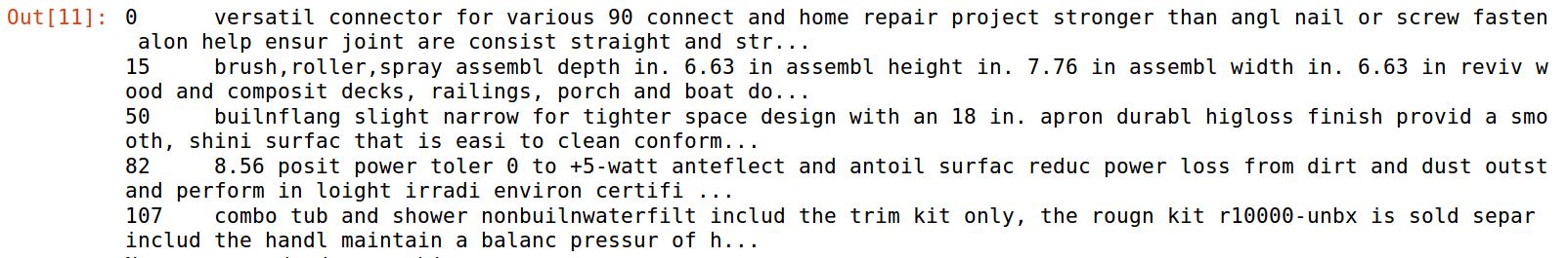
df.stemmed.head()
Scikit-learn provides two methods to get to our end result (a tf-idf weight matrix). One is a two-part process of using the CountVectorizer class to count how many times each term shows up in each document, followed by the TfidfTransformer class generating the weight matrix. The other does both steps in a single TfidfVectorizer class.
# Starting with the CountVectorizer/TfidfTransformer approach...
from sklearn.feature_extraction.text import CountVectorizer
from sklearn.feature_extraction.text import TfidfTransformer

cvec = CountVectorizer(stop_words='english', min_df=1, max_df=.5, ngram_range=(1,2))
cvec
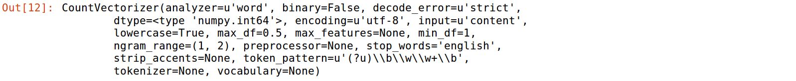
Let’s take a moment to describe these parameters as they are the primary levers for adjusting what feature set we end up with. First is “min_df” or mimimum document frequency. This sets the minimum number of documents that any term is contained in. This can either be an integer which sets the number specifically, or a decimal between 0 and 1 which is interpreted as a percentage of all documents. Next is “max_df” which similarly controls the maximum number of documents any term can be found in. If 90% of documents contain the word “spork” then it’s so common that it’s not very useful. Finally, we have “ngram_range” which is a tuple containing the range of ngram sizes to use. (1, 3) means use 1-grams, 2-grams, and 3-grams. We’re just using 1- and 2-grams.
After setting up our CountVectorizer, we follow the general fit/transform convention of scikit-learn, starting with fitting:
# Calculate all the n-grams found in all documents
from itertools import islice
cvec.fit(df.stemmed)
list(islice(cvec.vocabulary_.items(), 20))
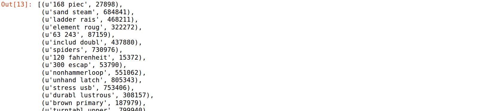
Let’s see how many unique 1- and 2-grams we get across all product documents…
# Check how many total n-grams we have
len(cvec.vocabulary_)
![]()
Ooof, too many. That’s way more products than we have, and the sparsity would likely be challenging for most models, if not just make the computation time much longer than necessary. Let’s try being more restrictive with the term selection (min_df = 0.25% of all documents and max_df = 10%)
# Check how many total n-grams we have
len(cvec.vocabulary_)
![]()
Ok, that’s more reasonable. It could turn out to be too few terms – before using for modeling we’ll want to determine how many product documents contain 0 of the terms identified – but it seems like a good starting point.
Our next move is to transform the document into a “bag of words” representation which essentially is just a separate column for each term containing the count within each document. After that, we’ll take a look at the sparsity of this representation which lets us know how many nonzero values there are in the dataset. The more sparse the data is the more challenging it will be to model, but that’s a discussion for another day.
cvec_counts = cvec.transform(df.stemmed)
print 'sparse matrix shape:', cvec_counts.shape
print 'nonzero count:', cvec_counts.nnz
print 'sparsity: %.2f%%' % (100.0 * cvec_counts.nnz / (cvec_counts.shape[0] * cvec_counts.shape[1]))

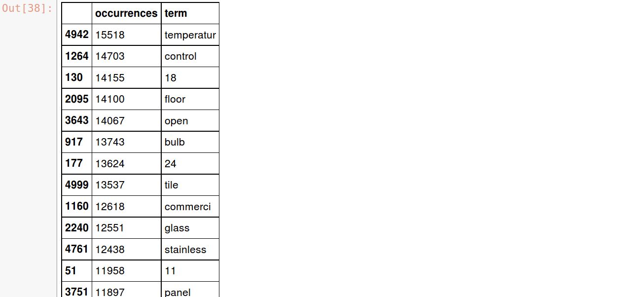
Let’s look at the top 20 most common terms
occ = np.asarray(cvec_counts.sum(axis=0)).ravel().tolist()
counts_df = pd.DataFrame({'term': cvec.get_feature_names(), 'occurrences': occ})
counts_df.sort_values(by='occurrences', ascending=False).head(20)
Now that we’ve got term counts for each document we can use the TfidfTransformer to calculate the weights for each term in each document
transformer = TfidfTransformer()
transformed_weights = transformer.fit_transform(cvec_counts)
transformed_weights

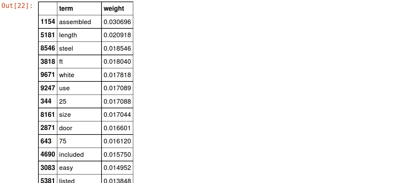
And we can take a look at the top 20 terms by average tf-idf weight
weights = np.asarray(transformed_weights.mean(axis=0)).ravel().tolist()
weights_df = pd.DataFrame({'term': cvec.get_feature_names(), 'weight': weights})
weights_df.sort_values(by='weight', ascending=False).head(20)
And that about wraps it up for Tf-idf calculation. As an example, you can jump straight to the end using the TfidfVectorizer class:
from sklearn.feature_extraction.text import TfidfVectorizer
tvec = TfidfVectorizer(min_df=.0025, max_df=.1, stop_words='english', ngram_range=ngramrange)
tvec_weights = tvec.fit_transform(df.stemmed.dropna())
weights = np.asarray(tvec_weights.mean(axis=0)).ravel().tolist()
weights_df = pd.DataFrame({'term': tvec.get_feature_names(), 'weight': weights})
weights_df.sort_values(by='weight', ascending=False).head(20)
In a future post, we’ll take a look at how to take this tf-idf weight matrix and feed it into a predictive model