In the last post we took a look at how reduce noisy variables from our data set using PCA, and today we’ll actually start modelling!
Random Forests are one of the easiest models to run, and highly effective as well. A great combination for sure. If you’re just starting out with a new problem, this is a great model to quickly build a reference model. There aren’t a whole lot of parameters to tune, which makes it very user friendly. The primary parameters include how many decision trees to include in the forest, how much data to include in each decision in the tree, and the stopping criteria for building each tree. You can tweak these values to predictably improve the score, but doing so comes with diminishing returns. For example, adding more trees to the forest will never make the score worse, but it will add computation time and may not make a dent in the accuracy. The next post will cover more about the parameters and how to tune them, but for now we’ll just use the default parameters with a few tweaks.
So, at this point we have a data set with a reasonably large number of features. The more features we have, the more likely it will be that we overfit the data, but there’s another way to continue to decrease the number of features we use. Yet another reason that the random forest model is great is that it automatically provides a measure of how important each feature is for classification. So we can fit a model with ALL the variables at first and then examine if any of the features are not particularly helpful.
The following code is a bit noisy, but we’re both determining the important features, and then sorting and plotting them to see what we can remove:
features_list = input_df.columns.values[1::]
X = input_df.values[:, 1::]
y = input_df.values[:, 0]

# Fit a random forest with (mostly) default parameters to determine feature importance
forest = RandomForestClassifier(oob_score=True, n_estimators=10000)
forest.fit(X, y)
feature_importance = forest.feature_importances_

# make importances relative to max importance
feature_importance = 100.0 * (feature_importance / feature_importance.max())

# A threshold below which to drop features from the final data set. Specifically, this number represents
# the percentage of the most important feature's importance value
fi_threshold = 15

# Get the indexes of all features over the importance threshold
important_idx = np.where(feature_importance > fi_threshold)[0]

# Create a list of all the feature names above the importance threshold
important_features = features_list[important_idx]
print "n", important_features.shape[0], "Important features(>", fi_threshold, "% of max importance):n",
        important_features

# Get the sorted indexes of important features
sorted_idx = np.argsort(feature_importance[important_idx])[::-1]
print "nFeatures sorted by importance (DESC):n", important_features[sorted_idx]

# Adapted from http://scikit-learn.org/stable/auto_examples/ensemble/plot_gradient_boosting_regression.html
pos = np.arange(sorted_idx.shape[0]) + .5
plt.subplot(1, 2, 2)
plt.barh(pos, feature_importance[important_idx][sorted_idx[::-1]], align='center')
plt.yticks(pos, important_features[sorted_idx[::-1]])
plt.xlabel('Relative Importance')
plt.title('Variable Importance')
plt.draw()
plt.show()

# Remove non-important features from the feature set, and reorder those remaining
X = X[:, important_idx][:, sorted_idx]
And this generates a chart something like this:
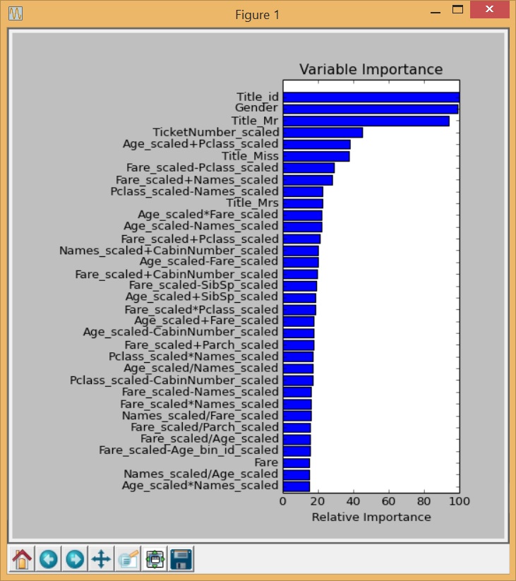
I’m sure you notice that the features look pretty odd. A lot of repetition of different combinations of the same few parameters. In this case, it makes sense that it would look like this, because we only have a few features that are appropriate for having automated feature generation applied. We do see that ALL of the original features are represented in some form within these synthetic features: gender, age, name, ticket, fare, passenger class, cabin, parent/children, and siblings/spouse. Is this the best approach for feature engineering for this problem, and RF in general? Almost certainly not, but for a lot of other problems this approach might prove very useful. Random Forests handle categorical data with no sweat, so converting that into different types of data and then generating features from it may not be required. I think actually in this case that using simple, unscaled variables would probably be better, as is evidenced by the fact that a much simpler feature set (such as Trevor Stephen’s R tutorial) did better than this one. At any rate, this gives an idea of the technique that can be used.
In the next post, we’ll look at techniques to automatically search for the best combination of model parameters.
Here are some good resources on Random Forests and Feature Importance you may enjoy:
- Random Forest discussion from Breiman and Cutler (the inventors)
- Scikit-learn’s RandomForestClassifier implementation
- A Gentle Introduction to Random Forests, Ensembles, and Performance Metrics in a Commercial System
- Variable Importance
Kaggle Titanic Tutorial in Scikit-learn
Part I – Intro
Part II – Missing Values
Part III – Feature Engineering: Variable Transformations
Part IV – Feature Engineering: Derived Variables
Part V – Feature Engineering: Interaction Variables and Correlation
Part VI – Feature Engineering: Dimensionality Reduction w/ PCA
Part VII – Modeling: Random Forests and Feature Importance
Part VIII – Modeling: Hyperparamter Optimization
Part IX – Bias, Variance, and Learning Curves
Part X – Validation: ROC Curves
Part XI – Summary